Warning: this tutorial is only available in English, even if you choose the French language at the bottom of the screen. Thank you for your understanding.
PUPAID: Pipeline for Unleashed Processing and Analysis of Immunofluorescence Data
PUPAID is a R + ImageJ package allowing to process immunofluorescence data and perform unsupervised analysis on it using a single cell contouring approach.

PUPAID could be in real life. Drawn by Craiyon.Table of contents
1) Prerequisites
1.1) R environment introduction and installation
To make the installation of R programming language and RStudio development software easier for new or beginner users, we highly recommend the following ressource, entitled « YaRrr! The Pirate’s Guide to R ». New users should at least read the first (« Preface ») and second (« Getting Started ») sections, as they provide clear and straightforward instructions on how to setup R and RStudio on Windows and MacOS operating systems. These sections will allow users to correctly install PUPAID and launch it flawlessly.
1.2) PUPAID R package installation
PUPAID package can be installed with the following command:
# The following line can be skipped if the devtools package is already installed

install.packages("devtools")

# Load the devtools package

library("devtools")

# Install PUPAID from GitHub repository

devtools::install_github("PaulRegnier/PUPAID")
1.3) Load PUPAID
To load PUPAID, simply enter the following command in the R console:
library("PUPAID")1.4) Update PUPAID
To update PUPAID, simply enter the following command in the R console:
devtools::install_github("PaulRegnier/PUPAID", force = TRUE)1.5) R Shiny interactive application
If one is not very familiar with programming and/or the R environment, PUPAID also provides an interactive application which uses the R shiny package. Once the package is installed (see previous section), users can launch the Shiny application with the following command:
PUPAID::interactivePUPAID()The process of launching PUPAID‘s interactive R Shiny application within RStudio can be visualized in the video below:
This facultative application totally replaces the successive R command which are detailed below, and helps users to keep the general PUPAID‘s workflow in mind during the processing and analysis steps. If desired, users can still use the traditionnal R commands, as the Shiny application is only a graphical way to launch the functions/scripts of interest within the R console.
From here, the rest of the workflow is pretty straightforward, as users only have to read and follow the steps indicated in the R Shiny window.
1.6) Example dataset
For learning and test purposes, PUPAID includes a dataset composed of 17 tiles (TIFF format) which contain demultiplexed signals of an 8-plex immunofluorescence staining performed using Opal technology from Akoya Biosciences, following their standard staining protocol. The staining was performed on a 5µm thick slide coming from FFPE-embedded salivary gland biopsy taken from a patient with Sjögren’s syndrome, and acquired with a Vectra Polaris scanner.
You can download these TIFF tiles as a single zip archive here (warning: the archive is about 1.16GB).
The staining panel (primarily designed to target and study the whole B and T cells compartments as well as several other features) was constructed as following:
- DAPI
- Anti-IL-21 (revealed with Opal 480)
- Anti-CD21 (revealed with Opal 520)
- Anti-TNFα (revealed with Opal 540)
- Anti-CD4 (revealed with Opal 570)
- Anti-IFNγ (revealed with Opal 620)
- Anti-CD27 (revealed with Opal 650)
- Anti-CD20 (revealed with Opal 690)
After acquisition, each of the generated tiles was demultiplexed using the InForm software coming with the Vectra Polaris acquisition software.
2) Workspace directory setup
PUPAID is designed to work in a self-organized set of directories, which can be created in the wd directory by running the following commands:
wd = file.path("YOUR PATH HERE")
setwd(wd)

PUPAID::createWorkspaceStructure(wd = wd)

imageJPath = file.path("YOUR ImageJ PATH HERE")
Please note that some functions of this workflow below need R to launch a macro script within ImageJ. In this fashion, all the generated macro codes throughout this workflow will be stored in the macros directory.
3) Pre-process data (optional)
In the case your data are in the form of contiguous and independent tiles, PUPAID allows to automatically rename and order them according to their ROI of origin, as well as stitch them into a single ROI. This is typically needed with data acquired using Vectra Polaris scanner, for instance.
Please note that for the code in this part to work, all the tiles should have the same dimensions, both in width and height.
In the case your data are in the form of full ROI containing the whole tissue or region you want to analyze, you can skip the section 3) and directly go to the section 4).
3.1) Generate a black tile
When data are acquired under the form of tiles, it is common to have regions that are not scanned (to limit as much as possible the acquisition time), thus leading to « holes » in the desired ROI, especially on the edges. To overcome this, PUPAID allows to generate a black tile (that is to say, devoid of any signal within each aquired channel) from an input tile located in the 1_generateBlackTile > input directory:
PUPAID::runMacro_generateBlackTile(imageJPath = imageJPath, wd = wd)Concretely, R will call ImageJ executable and launch in command line mode a macro already written for this purpose. The output black tile will be located in the 1_generateBlackTile > output directory.
3.2) Get the tile image size
Then, we need to extract the width and height (in µm) of a given tile:
imageSize = PUPAID::runMacro_getImageSize(imageJPath = imageJPath, wd = wd)These information will be necessary for the upcoming step.
Please note that this function will open the first tile it detects in the 1_generateBlackTile > output directory.
3.3) Rename and order tiles
Afterwards, one wants to automatically rename and order tiles to reconstitute their ROI of origin and prepare them for the future stitching:
renameAndOrderOutput = PUPAID::renameAndOrderTiles(AOI_x = imageSize[1], AOI_y = imageSize[2])The input tiles should be located in 2_renameAndOrderTiles > input directory.
This function will output renamed tiles, ordered by their ROI of origin (if applicable) in separate folders within the 2_renameAndOrderTiles > output directory.
3.4) Stitch tiles
Finally, PUPAID allows to stitch the renamed tiles together in order to generate full ROI embedded in a single image file:
PUPAID::stitchTiles(renameAndOrderOutput = renameAndOrderOutput, imageJPath = imageJPath, wd = wd)This function will stitch every tile present in the 2_renameAndOrderTiles > output directory and subdirectories. Concretely, R will call ImageJ executable and launch in command line mode a macro already written for this purpose. The final stitched images will then be located in the 3_stitchedTiles directory, as well as several other files: one text file per ROI regarding the tile configuration used by ImageJ for the actual stitching, and one global rds file named renameAndOrderOutput.rds containing the ROI information determined in the previous step.
4) Analysis
When your data are fully pre-processed (or if they do not need any pre-processing), PUPAID allows to analyze your ROI using a dedicated ImageJ macro.
4.1) Establish σ pairs to test
As PUPAID mainly bases its analysis on the Difference of Gaussians methodology for cell contour identification, one wants first to determine which pair of σ values could work best with the currently analyzed data (signal, tissue, etc.). To this, users can use the generateSigmaPairsList() function which will compute an approximative value for sigmaLow using an estimated overall diameter for the nuclei. Users only have to open their image of interest (or at least a cropped version of it) and to directly measure some nuclei in order to estimate an overall nuclei diameter (in µm).
This value will then be used as the radius parameter of the generateSigmaPairsList() function:
# Here, the 'radius' value is given as an example and should rather be determined by users

sigmaPairsToTest = PUPAID::generateSigmaPairsList(
    radius = 7.5,
    maxSigmaRatio = 2,
    step = 0.1
)
Concretely, the step parameter will be iteratively added to 1 (excluded) until the maxSigmaRatio limit is reached. In the example case above, the function will estimate the sigmaLow value to 2.13 (because of the radius set to 7.5), then will generate the following multiplicators: c(1.1, 1.2, 1.3, 1.4, 1.5, 1.6, 1.7, 1.8, 1.9, 2.0) and multiply them with the pre-determined sigmaLow value, thus leading to the following sigmaHigh values: c(2.343, 2.556, 2.769, 2.982, 3.195, 3.408, 3.621, 3.834, 4.047, 4.26). Ultimately, the function will return the following list of σ pairs to test:
[[1]]
[1] 2.130 2.343

[[2]]
[1] 2.130 2.556

[[3]]
[1] 2.130 2.769

[[4]]
[1] 2.130 2.982

[[5]]
[1] 2.130 3.195

[[6]]
[1] 2.130 3.408

[[7]]
[1] 2.130 3.621

[[8]]
[1] 2.130 3.834

[[9]]
[1] 2.130 4.047

[[10]]
[1] 2.13 4.26
Of note, users are still free to choose any σ pair they want/prefer for the upcoming analysis. To this, they just have to bypass the generateSigmaPairsList() function and directly generate a list of vectors of size 2 using the built-in R function list().
4.2) Benchmark σ pairs
Now, one wants to use the freshly generated sigmaPairsToTest list for the actual benchmarking of these σ pairs:
PUPAID::benchmarkSigmaPairs(imageJPath = imageJPath, wd = wd, sigmaPairsToTest = sigmaPairsToTest)This function takes a given image of interest located in the 4_testSigmaPair > input directory and outputs the resulting images in the 4_testSigmaPair > output directory.
Please note that the image given as input of this function should only have one channel (typically the one that should be used for cell segmentation). This can be easily achieved within ImageJ by converting the stack to images, then only saving as TIFF the channel to use for cell contour identification (typically DAPI). The final result is shown on the Figure 1 below.
To speed up the computation process, we recommand you to give to this function a cropped image which typically focuses on a densely infiltrated region of the tissue, or at least on a more or less representative section of the tissue. The Figure 2 and Figure 3 below show what can be expected before and after such cropping.

Figure 1 – DAPI only layer extracted from the stitched tile.

Figure 2 – DAPI only layer extracted from the stitched tile with a desired ROI for cropping.

Figure 3 – Cropped version of the DAPI only layer extracted from the stitched image.
This function produces for each given pair of σ values an image on which cell contours were determined using the same method as the real analysis performed in the next step. The function also outputs an ImageJ-formatted zip file containing all the segmented cell contours. The Figure 4 below summarizes all the output images produced with the previous code.

Figure 4 – Overview of the determination of cell contours using different pairs of σ values.
4.3) ROI analysis
When the best pair of σ values is empirically determined, one can proceed to the actual analysis on the full ROI containing all the desired channels:
# With this test dataset, it seems that sigmaLow = 2.13 and sigmaHigh = 2.982 values (making a ratio of 1:1.4) best determine cell contours

blockSize = 30
histogramBins = 256
maximumSlope = 3
sigmaLow = 2.13
sigmaHigh = 2.982

PUPAID::runMacro_analyzeROI(
    imageJPath = imageJPath,
    wd = wd,
    blockSize = blockSize,
    histogramBins = histogramBins,
    maximumSlope = maximumSlope,
    sigmaLow = sigmaLow,
    sigmaHigh = sigmaHigh
)
Basically, the final ImageJ analysis will take a given ROI located in the 5_analyzeROI > input directory and outputs the results in the 5_analyzeROI > output directory.
Regarding blockSize, histogramBins, and maximumSlope parameters, which are used by the CLAHE (Contrast Limited Adaptive Histogram Equalization) algorithm, the provided default values (blockSize = 30, histogramBins = 256, and maximumSlope = 3) should normally fit to most datasets. However, users can still change them if they know what they do. According to this page, the block size should be larger than the size of the features to be preserved, the number of histogram bins should not be greater than 256 and the maximum slope should not be too high but greater than 1.
Please note that because of some technical limitations, the macro itself (and thus the actual analysis of the image) cannot be launched directly within R. Instead, the runMacro_analyzeROI() function will only generate a ready-to-use macro which is launchable under ImageJ. Once the runMacro_analyzeROI() function has been executed, users should launch a fresh instance of ImageJ, then run Plugins > Macros > Run... within ImageJ and launch the edited macro of interest named 5_analyzeROI_run.txt and located in the macros directory.
Please note that this function can only process one ROI at a time, so you need to move the results at the end of each analysis before proceeding with a new one.
Simply follow the instructions as they are given during the execution of the macro.
Although the computations are fully automatized, the macro still needs the user input at several points:
- To rename each channel with a precise format:
MarkerName_FluorophoreOrColor_ImageJChannel- As a reminder, ImageJ uses this nomenclature to identify the channels:
c1 = red,c2 = green,c3 = blue,c4 = gray,c5 = cyan,c6 = magenta,c7 = yellow
- As a reminder, ImageJ uses this nomenclature to identify the channels:
- To choose the channel that will be used for cell contour identification
- To draw an additional ROI which contains background noise (for the Corrected Total Cell Fluorescence computation)
- To measure by any mean of choice the global tissue area (for estimation of cell counts per unit of area)
At the end, the macro will generate:
- Images with background-corrected and enhanced signals: 1 single TIFF file per available channel (whatever the provided image to analyze), as well as both composite and merged TIFF versions of the processed signals (only if there are between 1 and 7 channels included)
- TSV files (one per measured channel) where lines represent identified cells and columns show several features such as the fluorescence for the given channel (both MFI, integrated density and CTCF), area, coordinates of the centroid point and estimators of circularity and roundness, etc.
- A single zip file containing the ROI for each identified cell (for control and reproducibility purposes)
4.4) Transform TSV to XLSX
When the analysis has ended, all the ImageJ windows should automatically close. Here, one could desire to convert the freshly generated TSV files into XLSX files in order to be openable by Excel. This could be achieved with the following command:
PUPAID::convertTSVtoXLSX()Each TSV file will be converted into new XLSX files (and saved into the same directory), without erasing the original TSV files.
4.5) Transform TSV to FCS
Additionally, one wants to convert the freshly generated TSV files into a single FCS file:
PUPAID::mergeTSVtoFCS()This function takes all the TSV files found in the 5_analyzeROI > output directory and merges them into a single FCS file located in the same folder. This FCS file is ready to be imported and analyzed in any standard flow cytometry analysis softwares, such as FlowJo or Kaluza. This approach allows the user to spatially gate on cells of interest and directly look at the markers they express. Users can also use dedicated processing and analysis pipelines which handle FCS files, such as PICAFlow, cytofkit or CyTOF for instance.
At the end at this process, we invite users to move the results of the current analysis into another folder, especially if they have other ROI to analyze, as the analysis macro will overwrite anything stored in the 5_analyzeROI > output directory.
Of note, steps 4.2) through 4.4) (included) could be directly reperformed on another image of interest.
4.6) Visual analysis through conventional cytometry software
The FCS files produced by PUPAID are indeed intended to be opened and analyzed via third-party cytometry software like FlowJo or Kaluza, which will allow to visually and interactively explore the data and extract any relevant feature or measurement of choice. Interestingly, a full gating strategy is thus perfectly accessible with this approach, which will dramatically help to unlock the full potential of multiplex immunofluorescence data, as shown by the Figure 5 below.
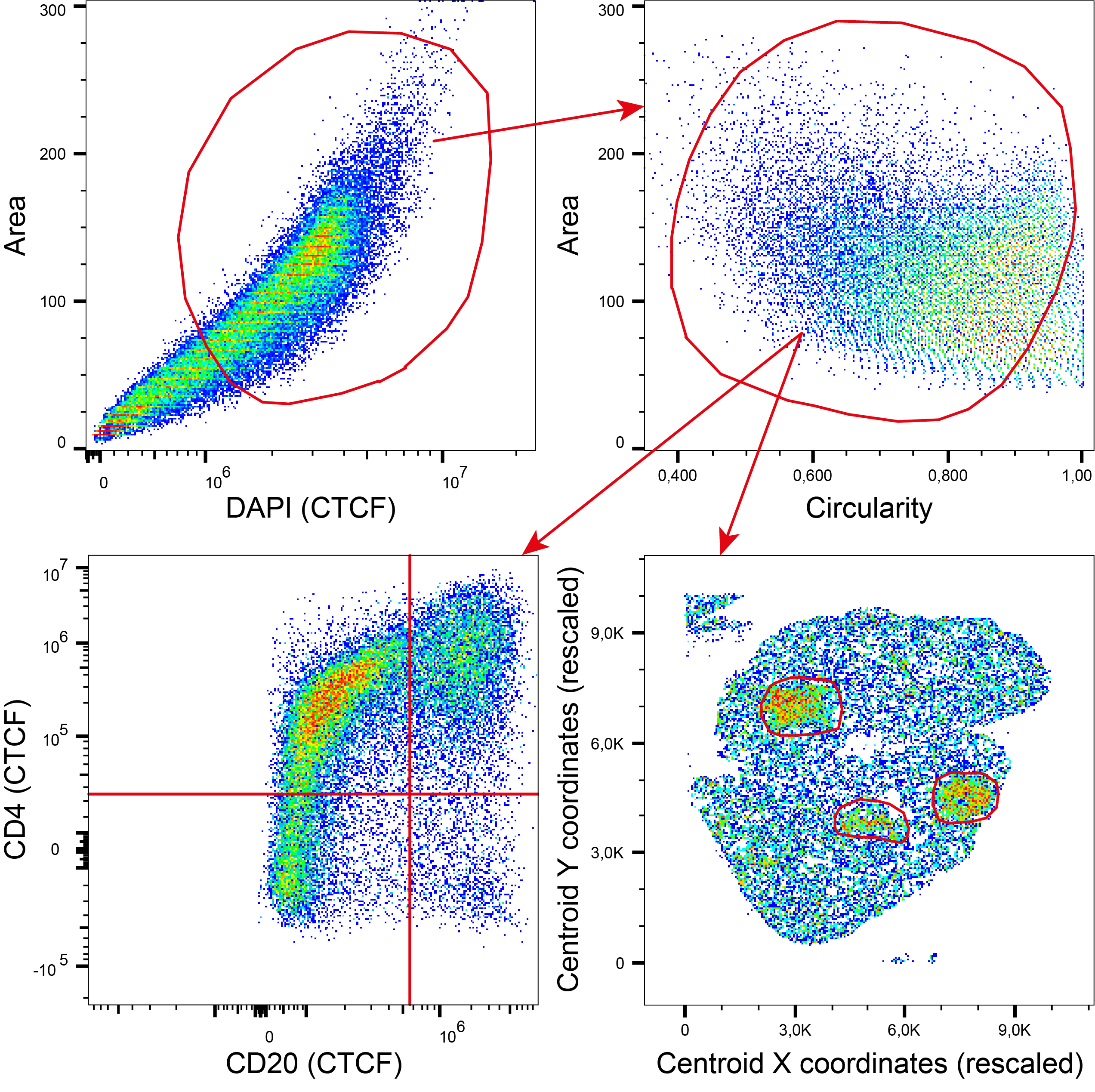
Figure 5 – Possible gating strategy to perform on FCS files generated by PUPAID.
5) Citation
If you used PUPAID in your analyses, please cite our article published in the PLOS One journal:
- PLOS One
- PubMed: 39298534
- DOI: 10.1371/journal.pone.0308970